Keras Tutorial - Traffic Sign Recognition
In this tutorial Tutorial assumes you have some basic working knowledge of machine learning and numpy. , we will get our hands dirty with deep learning by solving a real world problem. The problem we are gonna tackle is The German Traffic Sign Recognition Benchmark(GTSRB). The problem is to to recognize the traffic sign from the images. Solving this problem is essential for self-driving cars to operate on roads.
Representative images for each of the traffic sign classes in the GTSRB dataset
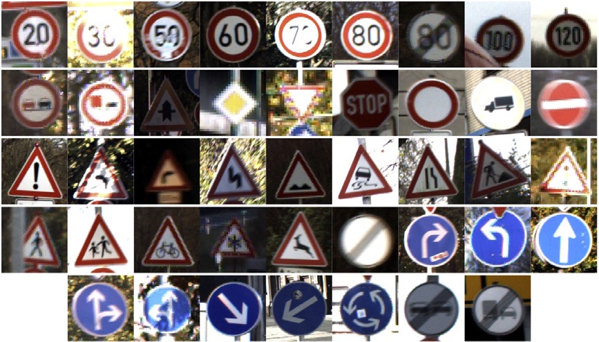
The dataset features 43 different signs under various sizes, lighting conditions, occlusions and is very similar to real-life data. Training set includes about 39000 images while test set has around 12000 images. Images are not guaranteed to be of fixed dimensions and the sign is not necessarily centered in each image. Each image contains about 10% border around the actual traffic sign.
Our approach to solving the problem will of course be very successful convolutional neural networks (CNNs). CNNs are multi-layered feed-forward neural networks that are able to learn task-specific invariant features in a hierarchical manner. You can read more about them in very readable Neural Networks and Deep Learning book by Michael Nielsen. Chapter 6 is the essential reading. Just read the first section in this chapter if you are in a hurry.
Note about the code: A recommended way to run the code in this tutorial and experiment with it is Jupyter notebook. A notebook with slightly improved code is available here.
We will implement our CNNs in Keras. Keras is a deep learning library written in python and allows us to do quick experimentation. Let’s start by installing Keras and other libraries: Protip: Use anaconda python distribution.
$ sudo pip install keras scikit-image pandas
Then download ‘Images and annotations’ for training and test set from GTSRB website and extract them into a folder. Also download ‘Extended annotations including class ids’ file for test set. Organize these files so that directory structure looks like this:
GTSRB
├── GT-final_test.csv
├── Final_Test
│   └── Images
└── Final_Training
    └── Images
        ├── 00000
        ├── 00001
        ├── ...
        ├── 00041
        └── 00042
Preprocessing
As you can see from the representative images above, images vary a lot in illumination. They also vary in size. So, let’s write a function to do histogram equalization in HSV color space and resize the images to a standard size:
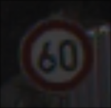
Input image to preprocess_img (scaled 4x)
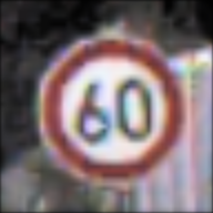
Processed image (scaled 4x)
import numpy as np
from skimage import color, exposure, transform

NUM_CLASSES = 43
IMG_SIZE = 48


def preprocess_img(img):
    # Histogram normalization in v channel
    hsv = color.rgb2hsv(img)
    hsv[:, :, 2] = exposure.equalize_hist(hsv[:, :, 2])
    img = color.hsv2rgb(hsv)

    # central square crop
    min_side = min(img.shape[:-1])
    centre = img.shape[0] // 2, img.shape[1] // 2
    img = img[centre[0] - min_side // 2:centre[0] + min_side // 2,
              centre[1] - min_side // 2:centre[1] + min_side // 2,
              :]

    # rescale to standard size
    img = transform.resize(img, (IMG_SIZE, IMG_SIZE))

    # roll color axis to axis 0
    img = np.rollaxis(img, -1)

    return img
Let’s preprocess all the training images are store into numpy arrays. We’ll also get labels of images from paths. We’ll convert targets to one-hot form as is required by keras:
from skimage import io
import os
import glob


def get_class(img_path):
    return int(img_path.split('/')[-2])

root_dir = 'GTSRB/Final_Training/Images/'
imgs = []
labels = []

all_img_paths = glob.glob(os.path.join(root_dir, '*/*.ppm'))
np.random.shuffle(all_img_paths)
for img_path in all_img_paths:
    img = preprocess_img(io.imread(img_path))
    label = get_class(img_path)
    imgs.append(img)
    labels.append(label)

X = np.array(imgs, dtype='float32')
# Make one hot targets
Y = np.eye(NUM_CLASSES, dtype='uint8')[labels]
Models
Let’s now define our models. We’ll use feed forward network with 6 convolutional layers followed by a fully connected hidden layer. We’ll also use dropout layers in between. Dropout regularizes the networks, i.e. it prevents the network from overfitting.
All our layers have relu activations except the output layer.
Output layer uses softmax activation as it has to output the probability for each of the classes.
Sequential is a keras container for linear stack of layers.
Each of the layers in the model needs to know the input shape it should expect,
but it is enough to specify input_shape for the first layer of the Sequential model.
Rest of the layers do automatic shape inference.
To attach a fully connected layer (aka dense layer) to a convolutional layer, we will have to reshape/flatten the output of the conv layer. This is achieved by Flatten layer
Go through the documentation of keras (relevant documentation : here and here) to understand what parameters for each of the layers mean.
from keras.models import Sequential
from keras.layers.core import Dense, Dropout, Activation, Flatten
from keras.layers.convolutional import Conv2D
from keras.layers.pooling import MaxPooling2D
from keras.optimizers import SGD
from keras import backend as K
K.set_image_data_format('channels_first')


def cnn_model():
    model = Sequential()

    model.add(Conv2D(32, (3, 3), padding='same',
                     input_shape=(3, IMG_SIZE, IMG_SIZE),
                     activation='relu'))
    model.add(Conv2D(32, (3, 3), activation='relu'))
    model.add(MaxPooling2D(pool_size=(2, 2)))
    model.add(Dropout(0.2))

    model.add(Conv2D(64, (3, 3), padding='same',
                     activation='relu'))
    model.add(Conv2D(64, (3, 3), activation='relu'))
    model.add(MaxPooling2D(pool_size=(2, 2)))
    model.add(Dropout(0.2))

    model.add(Conv2D(128, (3, 3), padding='same',
                     activation='relu'))
    model.add(Conv2D(128, (3, 3), activation='relu'))
    model.add(MaxPooling2D(pool_size=(2, 2)))
    model.add(Dropout(0.2))

    model.add(Flatten())
    model.add(Dense(512, activation='relu'))
    model.add(Dropout(0.5))
    model.add(Dense(NUM_CLASSES, activation='softmax'))
    return model
Before training the model, we need to configure the model the learning algorithm and compile it. We need to specify,
loss: Loss function we want to optimize. We cannot use error percentage as it is not continuous and thus non differentiable. We therefore use a proxy for it:categorical_crossentropyoptimizer: We use standard stochastic gradient descent with Nesterov momentum.metric: Since we are dealing with a classification problem, our metric is accuracy.
from keras.optimizers import SGD

model = cnn_model()

# let's train the model using SGD + momentum
lr = 0.01
sgd = SGD(lr=lr, decay=1e-6, momentum=0.9, nesterov=True)
model.compile(loss='categorical_crossentropy',
              optimizer=sgd,
              metrics=['accuracy'])
Training
Now, our model is ready to train.
During the training, our model will iterate over batches of training set, each of size batch_size.
For each batch, gradients will be computed and updates will be made to the weights of the network automatically.
One iteration over all the training set is referred to as an epoch.
Training is usually run until the loss converges to a constant.
We will add a couple of features to our training:
- Learning rate scheduler : Decaying learning rate over the epochs usually helps model learn better
- Model checkpoint : We will save the model with best validation accuracy. This is useful because our network might start overfitting after a certain number of epochs, but we want the best model.
These are not necessary but they improve the model accuracy.
These features are implemented via callback feature of Keras.
callback are a set of functions that will applied at given stages of training procedure like end of an epoch of training.
Keras provides inbuilt functions for both learning rate scheduling and model checkpointing.
from keras.callbacks import LearningRateScheduler, ModelCheckpoint


def lr_schedule(epoch):
    return lr * (0.1 ** int(epoch / 10))

batch_size = 32
epochs = 30

model.fit(X, Y,
          batch_size=batch_size,
          epochs=epochs,
          validation_split=0.2,
          callbacks=[LearningRateScheduler(lr_schedule),
                     ModelCheckpoint('model.h5', save_best_only=True)]
          )
You’ll see that model starts training and logs the losses and accuracies:
Train on 31367 samples, validate on 7842 samples
Epoch 1/30
31367/31367 [==============================] - 30s - loss: 1.1502 - acc: 0.6723 - val_loss: 0.1262 - val_acc: 0.9616
Epoch 2/30
31367/31367 [==============================] - 32s - loss: 0.2143 - acc: 0.9359 - val_loss: 0.0653 - val_acc: 0.9809
Epoch 3/30
31367/31367 [==============================] - 31s - loss: 0.1342 - acc: 0.9604 - val_loss: 0.0590 - val_acc: 0.9825
...
Now this might take a bit of time, especially if you are running on CPU. If you have a Nvidia GPU, you should install cuda. It speeds up the training dramatically. For example, on my Macbook air, it takes 10 minutes per epoch while on a machine with Nvidia Titan X GPU, it takes 30 seconds. Even modest GPUs offer impressive speedup because of the inherent parallelizability of the neural networks. This makes GPUs necessary for deep learning if anything big has to be done. Grab a coffee while you wait for training to complete ;).
Congratulations! You have just trained your first deep learning model.
Evaluation
Let’s quickly load test data and evaluate our model on it:
import pandas as pd
test = pd.read_csv('GT-final_test.csv', sep=';')

# Load test dataset
X_test = []
y_test = []
i = 0
for file_name, class_id in zip(list(test['Filename']), list(test['ClassId'])):
    img_path = os.path.join('GTSRB/Final_Test/Images/', file_name)
    X_test.append(preprocess_img(io.imread(img_path)))
    y_test.append(class_id)

X_test = np.array(X_test)
y_test = np.array(y_test)

# predict and evaluate
y_pred = model.predict_classes(X_test)
acc = np.sum(y_pred == y_test) / np.size(y_pred)
print("Test accuracy = {}".format(acc))
Which outputs on my system Results may change a bit because the weights of the neural network are randomly initialized.:
12630/12630 [==============================] - 2s
Test accuracy = 0.9792557403008709
97.92%! That’s sweet! It’s not far from average human performance (98.84%)[1].
A lot of things can be done to squeeze out extra performance from the neural net. I’ll implement one such improvement in the next section.
Data Augmentation
You might think 40000 images are a lot of images. Think about it again.
Our model has 1358155 parameters (try model.count_params() or model.summary()).
That’s 4X the number of training images.
If we can generate new images for training from the existing images, that will be a great way to increase the size of the dataset. This can be done by slightly
- translating of image
- rotating of image
- Shearing the image
- Zooming in/out of the image
Rather than generating and saving such images to hard disk, we will generate them on the fly during training. This can be done directly using built-in functionality of keras.
from keras.preprocessing.image import ImageDataGenerator
from sklearn.cross_validation import train_test_split

X_train, X_val, Y_train, Y_val = train_test_split(X, Y,
                                                  test_size=0.2, random_state=42)

datagen = ImageDataGenerator(featurewise_center=False,
                             featurewise_std_normalization=False,
                             width_shift_range=0.1,
                             height_shift_range=0.1,
                             zoom_range=0.2,
                             shear_range=0.1,
                             rotation_range=10.)

datagen.fit(X_train)

# Reinitialize model and compile
model = cnn_model()
model.compile(loss='categorical_crossentropy',
              optimizer=sgd,
              metrics=['accuracy'])

# Train again
epochs = 30
model.fit_generator(datagen.flow(X_train, Y_train, batch_size=batch_size),
                    steps_per_epoch=X_train.shape[0],
                    epochs=epochs,
                    validation_data=(X_val, Y_val),
                    callbacks=[LearningRateScheduler(lr_schedule),
                               ModelCheckpoint('model.h5', save_best_only=True)]
                    )
With this model, I get 98.29% accuracy on test set.
Frankly, I haven’t done much parameter tuning. I’ll make a small list of things which can be tried to improve the model:
- Try different network architectures. Try deeper and shallower networks.
- Try adding BatchNormalization layers to the network.
- Experiment with different weight initializations
- Try different learning rates and schedules
- Make an ensemble of models
- Try normalization of input images
- More aggressive data augmentation
This is but a model for beginners. For state of the art solutions of the problem, you can have a look at this, where the authors achieve 99.61% accuracy with a specialized layer called Spatial Transformer layer.
Conclusion
In this tutorial, we have learned how to use convolutional networks to solve a computer vision problem. We have used keras deep learning framework to implement convnets in python. We have achieved performance close to human level performance. We also have seen a way to improve the accuracy of the model: by augmentation of the training data.
References:
- Stallkamp, Johannes, et al. “Man vs. computer: Benchmarking machine learning algorithms for traffic sign recognition.” Neural networks 32 (2012): 323-332.