Self-Organized Criticality: An Explanation of 1/f Noise
Power law distribution is all around us, in cities, internet, genes, earthquakes and even brain. Physicists call this 1/f noise. This papers suggests a simple cellular automata model which can generate the power-law. Once the model evolves into a minimally stable state, it is said to be in self-organized criticality. From this state, small disturbances do nothing most of the time but sometimes create ‘black-swan’ avalanches which destroys the whole state.
Yellow highlights/annotations are my own. You can disable them.Abstract
We show that dynamical systems with spatial degrees of freedom naturally evolve into a self-organized critical point. Flicker noise, or $1/f$ noise, can be identified with the dynamics of the critical state. This picture also yields insight into the origin of fractal objects.
Paper
One of the classic problems in physics is the existence of the ubiquitous “$1/f$” noise which has been detected for transport in systems as diverse as resistors, the hour glass, the flow of the river Nile, and the luminosity of stars [1]. The low-frequency power spectra of such systems display a power-law behavior $f^{-\beta}$ over vastly different time scales. Despite much effort, there is no general theory that explains the widespread occurrence of $1/f$ noise.
Another puzzle seeking a physical explanation is the empirical observation that spatially extended objects, including cosmic strings, mountain landscapes, and coastal lines, appear to be self-similar fractal structures [2]. Turbulence is a phenomenon where self-similarity is believed to occur both in time and space. The common feature for all these systems is that the power-law temporal or spatial correlations extend over several decades where naively one might suspect that the physics would vary dramatically.
In this paper, we argue and demonstrate numerically that dynamical systems with extended spatial degrees of freedom naturally evolve into self-organized critical structures of states which are barely stable. We suggest that this self-organized criticality is the common underlying mechanism behind the phenomena described above. The combination of dynamical minimal stability and spatial scaling leads to a power law for temporal fluctuations. The noise propagates through the scaling clusters by means of a “domino” effect upsetting the minimally stable states. Long-wavelength perturbations cause a cascade of energy dissipation on all length scales, which is the main characteristic of turbulence.
The criticality in our theory is fundamentally different from the critical point at phase transitions in equilibrium statistical mechanics which can be reached only by tuning of a parameter, for instance the temperature. The critical point in the dynamical systems studied here is an attractor reached by starting far from equilibrium: The scaling properties of the attractor are insensitive to the parameters of the model. This robustness is essential in our explaining that no fine tuning is necessary to generate $1/f$ noise (and fractal structures) in nature.
Consider first a one-dimensional array of damped pendula, with coordinates $u_n$, connected by torsion springs that are weak compared with the gravitational force. There is an infinity of metastable or stationary states where the pendula are pointing (almost) down, $u_n \approx 2\pi N$, $N$ an integer, but where the winding numbers $N$ of the springs differ. The initial conditions are such that the forces $C_n = u_{n+1} - 2u_n + u_{n-1}$, are large, so that all the pendula are unstable. The pendula will rotate until they reach a state where the spring forces on all the pendula assume a large value $\pm K$ which is just barely able to balance the gravitational force to keep the configuration stable. If all forces are initially positive, then the final forces will all be $K$. Of course, the array is also stable in any configuration where the springs are still further relaxed; however, the dynamics stops upon reaching this first, maximally sensitive state. We call such a state locally minimally stable.[3]
What is the effect of small perturbations on the minimally stable structure? Suppose that we “kick” one pendulum in the forward direction, relaxing the force slightly. This will cause the force on a nearest-neighbor pendulum to exceed the critical value and the perturbation will propagate by a domino effect until it hits the end of the array. At the end of this process the forces are back to their original values, and all pendula have rotated one period. Thus, the system is stable with respect to small perturbations in one dimension and the dynamics is trivial.
The situation is dramatically different in more dimensions. Naively, one might expect that the relaxation dynamics will take the system to a configuration where all the pendula are in minimally stable states. A moment’s reflection will convince us that it cannot be so. Suppose that we relax one pendulum slightly; this will render the surrounding pendula unstable, and the noise will spread to the neighbors in a chain reaction, ever amplifying since the pendula generally are connected with more than two minimally stable pendula, and the perturbation eventually propagates throughout the entire lattice. This configuration is thus unstable with respect to small fluctuations and cannot represent an attracting fixed point for the dynamics. As the system further evolves, more and more more-than-minimally stable states will be generated, and these states will impede the motion of the noise. The system will become stable precisely at the point when the network of minimally stable states has been broken down to the level where the noise signal cannot be communicated through infinite distances. At this point there will be no length scale in the problem so that one might expect the formation of a scale-invariant structure of minimally stable states. Hence, the system might approach, through a self-organized process, a critical point with power-law correlation functions for noise and other physically observable quantities. The “clusters” of minimally stable states must be defined dynamically as the spatial regions over which a small local perturbation will propagate. In a sense, the dynamically selected configuration is similar to the critical point at a percolation transition where the structure stops carrying current over infinite distances, or at a second-order phase transition where the magnetization clusters stop communicating. The arguments are quite general and do not depend on the details of the physical system at hand, including the details of the local dynamics and the presence of impurities, so that one might expect self-similar fractal structures to be widespread in nature: The “physics of fractals”[4] could be that they are the minimally stable states originating from dynamical processes which stop precisely at the critical point.
The scaling picture quite naturally gives rise to a power-law frequency dependence of the noise spectrum. At the critical point there is a distribution of clusters of all sizes; local perturbations will therefore propagate over all length scales, leading to fluctuation lifetimes over all time scales. A perturbation can lead to anything from a shift of a single pendulum to an avalanche, depending on where the perturbation is applied. The lack of a characteristic length leads directly to a lack of a characteristic time for the resulting fluctuations. As is well known, a distribution of lifetimes $D(t) \sim t^{-a}$ leads to a frequency spectrum
\[S(\omega) = \int dt \frac{tD(t)}{1 + (wt)^2} \approx \omega^{-2 + a}\]In order to visualize a physical system expected to exhibit self-organized criticality, consider a pile of sand. If the slope is too large, the pile is far from equilibrium, and the pile will collapse until the average slope reaches a critical value where the system is barely stable with respect to small perturbations. The “$1/f$” noise is the dynamical response of the sandpile to small random perturbations.
To add concreteness to these considerations we have performed numerical simulations in one, two, and three dimensions on several models, to be described here and in forthcoming papers. One model is a cellular automaton, describing the interactions of an integer variable $z$ with its nearest neighbors. In two dimensions $z$ is updated synchronously as follows:
\[z(x, y) \longrightarrow z(x, y) - 4,\] \[z(x \pm 1, y) \longrightarrow z(x \pm 1, y) +1,\] \[z(x, y \pm 1) \longrightarrow z(x, y \pm 1) +1,\]if $z$ exceeds a critical value $K$. There are no parameters since a shift in $K$ simply shifts $z$. Fixed boundary conditions are used, i.e., $z=0$ on boundaries. The cellular variable may be thought of as the force on an individual pendulum, or the local slope of the sand pile (the “hour glass”) in some direction. If the force is too large, the pendulum rotates (or the sand slides), relieving the force but increasing the force on the neighbors. The system is set up with random initial conditions $z \gg K$, and then simply evolves until it stops, i.e., all $z$’s are less than $K$. The dynamics is then probed by measurement of the response of the resulting state to small local random perturbations. Indeed, we found response on all length scales limited only by the size of the system.
Figure 1: Self-organized critical state of minimally stable clusters, for a $100 \times 100$ array.
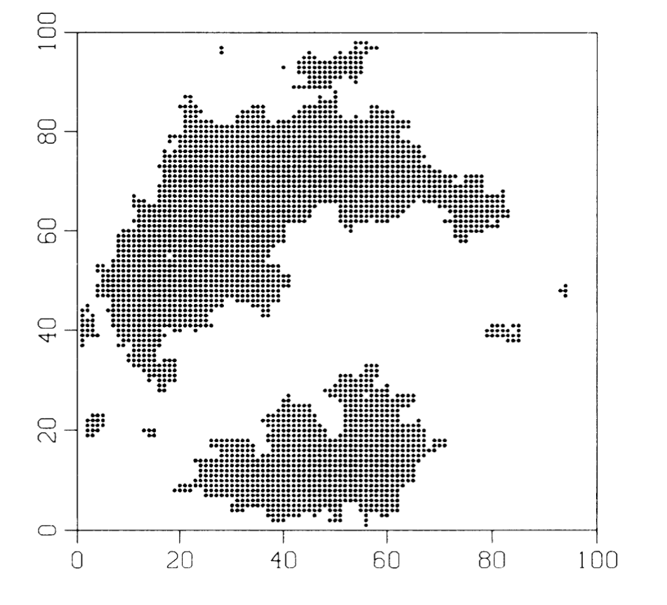
Figure 1 shows a structure obtained for a two-dimensional array of size $100 \times 100$. The dark areas indicate clusters that can be reached through the domino process originated by the tripping of only a single site. The clusters are thus defined operationally – in a real physical system one should perturb the system locally in order to measure the size of a cluster. Figure 2(a) shows a log-log plot of the distribution $D(s)$ of cluster sizes for a two-dimensional system determined simply by our counting the number of affected sites generated from a seed at one site and averaging over many arrays. The curve is consistent with a straight line, indicating a power law $D(s) \sim s^{-\tau}, \tau \approx 0.98$. The fact that the curve is linear over two decades indicates that the system is at a critical point with a scaling distribution of clusters.
Figure 2: Distribution of cluster sizes at criticality in two and three dimensions, computed dynamically as described in the text. (a) $50 \times 50$ array, averaged over 200 samples; (b) $20 \times 20 \times 20$ array, averaged over 200 samples. The data have been coarse grained.
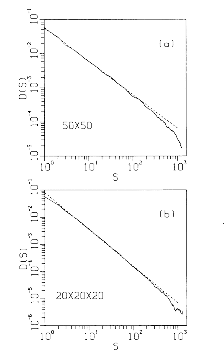
Figure 2(b) shows a similar plot for a three-dimensional array, with an exponent of $\tau \approx 1.35$. At small sizes the curve deviates from the straight line because discreteness effects of the lattice come into play. The falloff at the largest cluster sizes is due to finite-size effects, as we checked by comparing simulations for different array sizes.[5]
A distribution of cluster sizes leads to a distribution of fluctuation lifetimes. If the perturbation grows with an exponent $\gamma$ within the clusters, the lifetime $t$ of a cluster is related to its size $s$ by $\tau ^ {1 + \gamma} \approx s$. The distribution of lifetimes, weighted by the average response $s/t$, can be calculated from the distribution of cluster sizes:
\[D(t) = \frac{s}{t} D(s(t)) \frac{ds}{dt} \approx t^{-(\gamma + 1)\tau + 2 \gamma} \equiv t ^ {-\alpha} \tag{2}\]
Figure 3: Distribution of lifetimes corresponding to Fig. 2. (a) For the $50 \times 50$ array, the slope $\alpha \approx 0.42$, yielding a “$1/f$” noise spectrum $f^{-1.58}$; (b) $20 \times 20 \times 20$ array, $\alpha \approx 0.90$, yielding an $f^{-1.1}$ spectrum
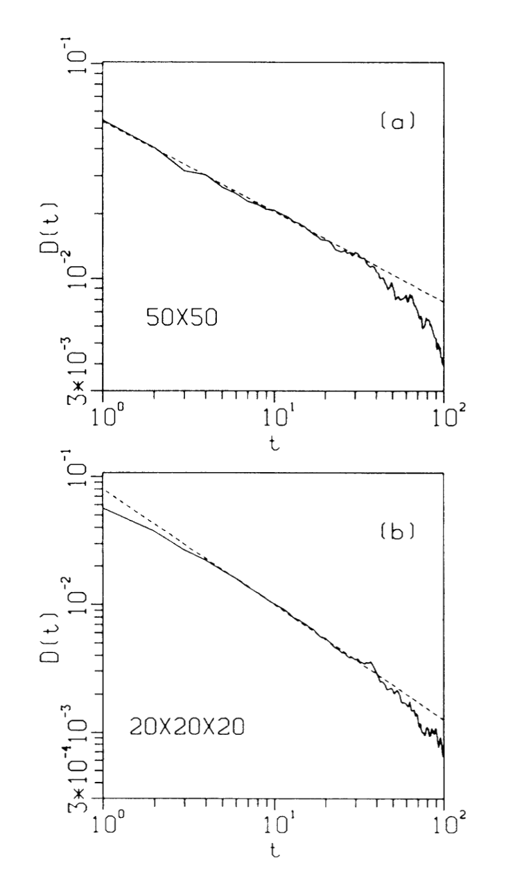
Figure 3 shows the distribution of lifetimes corresponding to Fig. 2 (namely how long the noise propagates after perturbation at a single site, weighted by the temporal average of the response). This leads to another line indicating a distribution of lifetimes of the form (2) with $\alpha \approx 0.42$ in two dimensions ($50 \times 50$), and $\alpha \approx 0.90$ in three dimensions. These curves are less impressive than the corresponding cluster-size curves, in particular in three dimensions, because the lifetime of a cluster is much smaller than its size, reducing the range over which we have reliable data. The resulting power-law spectrum is $S(\omega) \approx \omega^{-2 + \alpha} \approx \omega^{-1.58}$ in 2D and $\omega^{-1.1}$ in 3D.
To summarize, we find a power-law distribution of cluster sizes and time scales just as expected from general arguments about dynamical systems with spatial degrees of freedom. More numerical work is clearly needed to improve accuracy, and to determine the extent to which the systems are “universal,” e.g., how the exponents depend on the physical details. Our picture of $1/f$ spectra is that it reflects the dynamics of a self-organized critical state of minimally stable clusters of all length scales, which in turn generates fluctuations on all time scales. Voss and Clarke [6] have performed measurements indicating that the noise at a given frequency $f$ is spatially correlated over a distance $L(f)$ which increases as $f$ decreases. We urge that more experiments of this type be performed to investigate the scaling proposed here.
We believe that the new concept of self-organized criticality can be taken much further and might be the underlying concept for temporal and spatial scaling in a wide class of dissipative systems with extended degrees of freedom.
We thank George Reiter for suggesting that these ideas might apply to the problem of turbulence. This work was supported by the Division of Materials Sciences, U. S. Department of Energy, under Contract No. DE-AC02-76CH00016.
References
- For a review of 1/f noise in astronomy and elsewhere, see W.H. Press, Commun. Mod. Phys. C 7, 103 (1978).
- B. Mandelbrot, The Fractal Geometry of Nature (Freeman, San Francisco, 1982).
- C. Tang, K. Wiesenfeld, P. Bak, S. Coppersmith, and P. Littlewood, Phys. Rev. Lett. 58, 1161 (1987).
- L. P. Kadanoff, Phys. Today 39, No. 2, 6 (1986).
- P. Bak, C. Tang, and K. Wiesenfeld, to be published.
- R. F. Voss and J. Clarke, Phys. Rev. B 13, 556 (1976).