Deep Learning Crash Course Part 1
Deep learning is the thing in machine learning these days. I probably don’t need to explain you the reason for buzz. This series of posts is a yet another attempt to teach deep learning.
My aim here is to
- Explain all the basics and practical advice you need
- This should be readable in less than 2/3 hours
Obviously, I assume a few things about your knowledge:
- You know basic machine learning; you know what training, validation and test sets are.
- You know calculus and about gradients. I recap them anyway though.
I divide the crash course into two parts for convenience:
- Part 1: Recap of calculus, gradient descent and neural networks
- Part 2: CNNs, tricks, practical advice
A printable version is available here Tex source is here. .
We will start with basics of optimization.
Calculus: Recap
Let’s recap what a derivative is.
Derivative
Derivative of function $f(v)$ ($f’(v)$ or $\frac{df}{dv}$) measures sensitivity of change in $f(v)$ with respect of change in $v$.
Figure: Derivative illustration. Red is for positive $v$ direction and green is for negative $v$ direction. Source.
Direction (i.e sign) of the derivative at a points gives the direction of (greatest) increment of the function at that point.
Gradient
The gradient is a multi-variable generalization of the derivative. It is a vector valued function. For function $f(v_1, v_2, \ldots, v_n)$, gradient is a vector whose components are $n$ partial derivatives of $f$:
\[\nabla f = (\frac{\partial f}{\partial v_1 }, \frac{\partial f}{\partial v_2 }, \ldots, \frac{\partial f}{\partial v_n })\]Figure: Gradient of the 2D function $f(x, y) = xe^{−(x^2 + y^2)}$ is plotted as blue arrows over the pseudocolor (red is for high values while blue is for low values) plot of the function. Source.
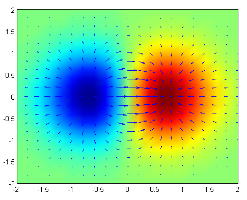
Similar to derivative, direction of the gradient at a point is the steepest ascent of the function starting from that point.
Optimization
Given a function $C(v_1, v_2, \ldots, v_n)$, how do we optimize it? i.e, find a point which minimizes this function globally.
This is a very generic problem; lot of practical and theoretical problems can be posed in this form. So, there is no general answer.
Gradient Descent
However, for a class of functions called convex functions, there is a simple algorithm which is guaranteed to converge to minima. Convex functions have only one minima. They look something like this:
Figure: A 2d convex function. Source.
To motivate our algorithm, imagine this function as a valley and a ball is put at a random point on the valley and allowed to roll. Our common sense tells that ball will eventually roll to the bottom of the valley.
Figure: Gradient descent illustration: a ball on a valley. Source
Let’s roughly simulate the motion of the ball! Key observation is that the ball moves in the steepest direction of descent. This is negative Gradient gives us steepest direction of ascent. of the gradient’s direction.
Great! Let’s put together our algorithm:
Algorithm: Gradient Descent
- Start at a random point: $v$
- While $v$ doesn’t converge do
- Update $v$ in the direction of steepest descent: $v \rightarrow v’ = v -\eta \nabla C$
- end while
Figure: Gradient descent on a series of level sets. Source.

Here $\eta$ is called learning rate. If it is too small, algorithm can be very slow and might take too many iterations to converge. If it is too large, algorithm might not even converge.
Example: Regression
Let’s apply the things learnt above on linear regression problem. Here’s a recap of linear regression:
Our model is $y(x) = wx + b$. Parameters are $v = (w, b)$ We are given training pairs $(x^1, y^1), (x^2, y^2), \ldots, (x^n, y^n)$.
Notation clarifiction: Here, superscripts are indices, not powers
We want to find $w$ and $b$ which minimize the following cost/loss function:
\[C(w, b) = \frac{1}{n} \sum_{i = 1}^{n} C_i(w, b) = \frac{1}{2n} \sum_{i = 1}^{n} \| y(x^i) - y^i\|^2\]where $C_i(w, b) = \frac{1}{2} | y(x^i) - y^i|^2 = \frac{1}{2} | wx^i + b - y^i|^2$ is the loss of the model for $i$ th training pair.
Let’s calculate gradients,
\[\nabla C = \frac{1}{n} \sum_{i = 1}^{n} \nabla C_i\]where $\nabla C_i$ is computed using:
\[\nabla C_i = \left( \frac{\partial C_i}{\partial w}, \frac{\partial C_i}{\partial b} \right) = \left( (wx^i + b - y^i)x^i, (wx^i + b - y^i) \right)\]Update rule is
\[v \rightarrow v' = v -\eta \nabla C = v -\frac{\eta}{n} \sum_{i = 1}^{n} \nabla C_i\]Stochastic Gradient Descent
In the above example, what if we have very large number of samples i.e $n \gg 0$? At every optimization step, we have to compute $\nabla C_i$ for each sample $i = 1, 2, \ldots, n$. This can be very time consuming!
Can we approximate $\nabla C$ with a very few samples? Yes!
\[\nabla C = \frac{1}{n} \sum_{i = 1}^{n} \nabla C_i \approx \frac{1}{m} \sum_{j \in S_m} \nabla C_j\]where $S_m$ is random subset of size $m \ll n$ of ${1, 2, \ldots,n}$. It turns out that this approximation, even though estimated only from a small random subset of samples, is good enough for convergence of gradient descent. This subset of data is called minibatch and this technique is called stochastic gradient descent.
Then stochastic gradient descent works by picking a randomly chosen subset of data and trains (i.e updates $v$) with gradient approximation computed from them. Next, another subset is picked up and trained with them. And so on, until we’ve exhausted all the training data, which is said to complete an epoch of training. Concretely, following is the stochastic gradient descent algorithm.
Algorithm: Stochastic Gradient Descent
For a fixed number of epochs, repeat:
- Randomly partition the data into minibatches each of size $m$
- For each minibatch $S_m$ repeat:
- Update the parameters using
Neural Networks
With this background, we are ready to start with neural networks.
Perceptron
Perceptron, a type of artificial neuron was developed in the 1950s and 1960s. Today, it’s more common to use Rectified Linear Units (ReLUs). Nevertheless, it’s worth taking time to understand the older models.
So how do perceptrons work? A perceptron takes several inputs, $x_1, x_2, \ldots x_n$ and produces a single output:
Figure: Perceptron Model. Source.
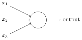
Weights $w_1, w_2, \ldots w_n$ decide the importance of each of the inputs on output $y(x)$. There is also a threshold $b$ to decide the output. These are the parameters of the model.
The expression of the output is
\[y(x) = \sigma\left(\sum_j w_j x_j - b\right)\]where $\sigma(z)$ is step function, \(\begin{eqnarray} \sigma(z) & = & \left\{ \begin{array}{ll} 0 & \mbox{if } z \leq 0 \\ 1 & \mbox{if } z > 0 \end{array} \right. \end{eqnarray}\)
Therefore \(\begin{eqnarray} y(x) & = & \left\{ \begin{array}{ll} 0 & \mbox{if } \sum_j w_j x_j \leq b \\ 1 & \mbox{if } \sum_j w_j x_j > b \end{array} \right. \end{eqnarray}\)
That’s the basic mathematical model. A way you can think about the perceptron is that it’s a device that makes decisions by weighing up evidence. An example:
Example: Perceptron and decision-making. Straight from here.
Suppose the weekend is coming up, and you’ve heard that there’s going to be a cheese festival in your city. You like cheese, and are trying to decide whether or not to go to the festival. You might make your decision by weighing up three factors:
- Is the weather good?
- Does your boyfriend or girlfriend want to accompany you?
- Is the festival near public transit? (You don’t own a car).
We can represent these three factors by corresponding binary variables \(x1\), \(x2\) and \(x_3\)
Now, suppose you absolutely adore cheese, so much so that you’re happy to go to the festival even if your boyfriend or girlfriend is uninterested and the festival is hard to get to. But perhaps you really loathe bad weather, and there’s no way you’d go to the festival if the weather is bad. You can use perceptrons to model this kind of decision-making.
You can use perceptrons to model this kind of decision-making. One way to do this is to choose a weight $w_1=6$ for the weather, and $w_2=2$ and $w_3=2$ for the other conditions and threshold (or more aptly, bias) term $b = 5$. By varying the weights and the threshold, we can get different models of decision-making.
Another way perceptrons can be used is to compute the elementary logical functions we usually think of as underlying computation, functions such as AND, OR, and NAND. Check that following perceptron implements NAND:
Figure: NAND implemented by perceptron. Source.
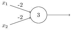
If you are familiar with digital logic, you will know that NAND gate is a universal gate. That is, any logical computation can be computed using just NAND gates. Then, the same property follows for perceptrons.
Multi Layer Perceptrons and Sigmoid
Although perceptron isn’t a complete model of human decision-making, the above example illustrates how a perceptron can weigh up different kinds of evidence in order to make decisions. And it should seem plausible that a complex network of perceptrons could make quite subtle decisions
Figure: Multi layer perceptron. Source.
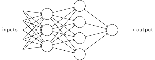
This network is called Multi layered perceptron (MLP). In this MLP, the first column of perceptrons - what we’ll call the first layer of perceptrons - is making three very simple decisions, by weighing the input evidence. What about the perceptrons in the second layer? Each of those perceptrons is making a decision by weighing up the results from the first layer of decision-making. In this way a perceptron in the second layer can make a decision at a more complex and more abstract level than perceptrons in the first layer. And even more complex decisions can be made by the perceptron in the third layer. In this way, a many-layer network of perceptrons can engage in sophisticated decision making.
How do we learn the parameters of the above model? Gradient Descent! MLP model is far from convex. Therefore, gradient descent is not guaranteed to converge! But it turns out that it works fine with a few tweaks which we describe below. However, the network is very discontinuous. In fact, a small change in the weights or bias of any single perceptron in the network can sometimes cause the output of that perceptron to completely flip, say from 0 to 1. This makes it very difficult for gradient descent to converge.
How do we overcome this? What is the source of this discontinuity? Remember that output of perceptron is given by $y(x) = \sigma\left(\sum_j w_j x_j - b\right)$ where $\sigma(z)$ is step function \(\begin{eqnarray} \sigma(z) & = & \left\{ \begin{array}{ll} 0 & \mbox{if } z \leq 0 \\ 1 & \mbox{if } z > 0 \end{array} \right. \end{eqnarray}\). This $\sigma(z)$ is the source of discontinuity. Can we replace step function with a smoother version of it?
Check out the following function:
\[\begin{eqnarray} \sigma(z) = \frac{1}{1+e^{-z}}. \end{eqnarray}\]If you graph it, it’s quite clear that this function is smoothed out version of a step function. This function is called sigmoid.
Figure: Sigmoid function. When $z$ is large and positive, Then $e^{-z} \approx 0$ and so $\sigma(z) \approx 1$. Suppose on the other hand that $z$ is very negative. Then $e^{-z} \rightarrow \infty$, and $\sigma(z) \approx 0$.
Source.

With the sigmoid neuron, gradient descent usually converges. Before computing gradients for gradient descent, we need to discuss loss functions I use terms loss function and cost function interchangeably. and activation functions.
ReLU Activation
By now, you have seen that general form of a artificial neuron is $y(x) = \sigma\left(\sum_j w_j x_j - b\right)$. Here the function $\sigma(z)$ is called activation function. So far, we have seen two different activations:
- Step function
- Sigmoid function
Let me introduce another activation function, rectifier or rectified linear unit (ReLU):
\[\sigma(z) = \max(0, z)\]Its graph looks like this:
Figure: ReLU.
Source.

Because of reasons we describe later More specifically, because of vanishing and exploding gradients problem. Read more here , ReLUs are preferred activation functions these days. You will almost never see sigmoid activation function in modern deep neural networks.
Loss functions
To train any machine learning model, we need to measure how well the model fits to training set. Such a function is called loss/cost function. In the regression problem we discussed before, cost function was $C(w, b) = \frac{1}{2n} \sum_{i = 1}^{n} | y(x^i) - y^i|^2$. Minimizing the cost function trains the model.
We will make two assumptions about our cost function:
- The cost function can be written as an average over cost functions $C_i$ for individual training examples, $(x^i, y^i)$. i.e, $C = \frac{1}{n} \sum_{i = 1}^{n} C_i$
- Cost can be written as a function of the outputs from the neural network. i.e, $C_i = L(y(x^i), y^i)$ where $y(x)$ is the output from the network.
In the case of regression, we used $L_2$ loss, $L(o, y) = \frac{1}{2} | o - y|^2$. We could have also used $L_1$ loss, $L(o, y) = | o - y |_{L_1}$.
Cross Entropy Loss
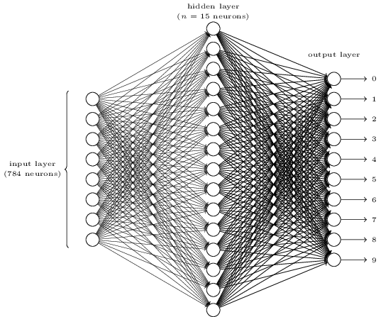
What if we have a classification problem? What loss do we use? Consider the following MLP for digit classification:
Figure: MLP for digit classification.
Source.
Here, we have output $o$ of size 10 and a target class $y$. We could have used $L_1(o, e_y)$ or $L_2(o, e_y)$ loss where $e_y$ is $y$th standard unit vector. But it turns out that this doesn’t work very well.
Instead, We will consider the outputs as a probability distribution over 10 classes and use what is called a cross entropy loss:
\[L(o, y) = - \log(o_y)\]To understand this function, realize that $o_y$ is the output probability of the target class $y$. Minimizing negative of log of this probability, maximizes the probability. Also, $L \geq 0$ because $\log(x) < 0$ for $x \in [0, 1]$.
Softmax Activation
If we use cross entropy loss, we cannot use sigmoids as activations of output layer because sigmoids do not guarantee a probability distribution. This is because, although each component of the output is in $[0, 1]$, they need not add up to 1.
We therefore use an activation layer/function called softmax. According to this function, the activation $a_j$ of the $j$th output neuron is
\[a_j = \frac{e^{z_j}}{\sum_k e^{z_k}}\]where in the denominator we sum over all the output neurons.
This expression may seem opaque if you are not familiar with it. Observe the following:
- Activations are positive: $a_j \geq 0$
- Activations sum to 1: $\sum_j a_j = 1$
- If you increase $z_m$ keeping others constant, $a_m$ increases. Other activations decrease to ensure that the sum remains 1.
- If $z_m$ is much larger than the others, $a_m \approx 1$ and $a_k \approx 0$ for $k \neq m$.
Therefore softmax is a probability distribution which behaves like smooth version of argmax.
Backpropogation
We have so far discussed the model component of neural networks. We haven’t yet discussed how we learn the parameters of the networks i.e, weights and biases of the layers.
As expected, we will use stochastic gradient descent. For this, we need gradients of $C_i$, loss for the $i$th training example, with respect to all the parameters of network. Computation of this quantity, $\nabla C_i$ is slightly involved. Let’s start with writing the expression for $C_i$. Let’s represent all the parameters of the network with $\theta$:
\[C_i(\theta) = L\left(y(x^i, \theta), y^i \right)\]Let’s break the above function into composition of layers (or functions in general)
\[C = f_L \circ \ f_{L-1} \circ \cdots \circ f_l \circ \cdots \circ f_1\]
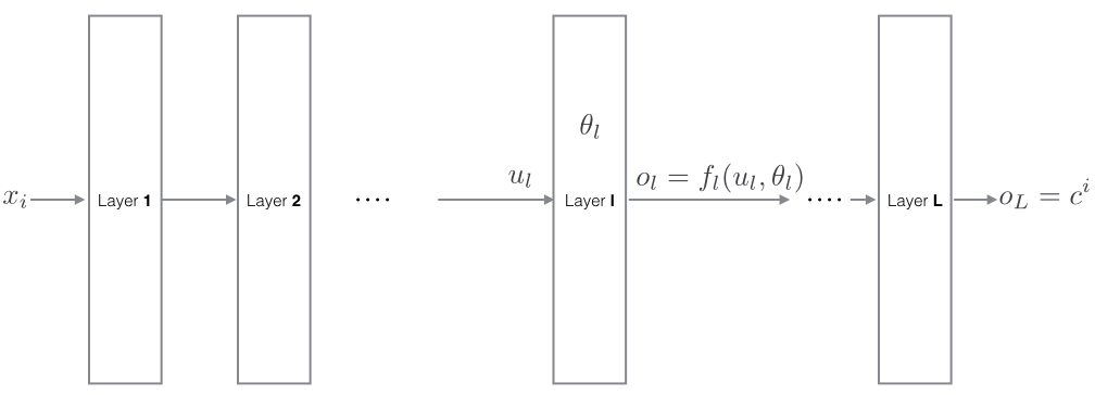
Here, $l$th In particular, $C = o_L = y_L(u_L) = L(u_L, y^i)$ layer/function takes in input $u_l$ and outputs
\[o_l = f_l(u_l, \theta_l) \tag{1}\]where $\theta_l$ are learnable parameters of this layer. Since output of $l-1$th layer is fed to $l$ th layer as input,
\[u_l = o_{l-1} \tag{2}\]We require $\nabla C = \left(\frac{\partial C}{\partial\theta_1}, \frac{\partial C}{\partial\theta_2}, \ldots, \frac{\partial C}{\partial\theta_L}\right)$. Therefore, we need to compute
\[\frac{\partial C}{\partial\theta_l} = \frac{\partial o_L}{\partial\theta_l} \text{ for } l = 1, 2, \dots n\]To compute this quantity, we will compute generic You will see ahead why this quantity is useful. :
\[\frac{\partial o_m}{\partial \theta_l}\]Before getting started, let’s write down the chain rule. Chain rule is the underlying operation of our algorithm.
For function f(x, y),
\[\frac{\partial f}{\partial t} = \frac{\partial f}{\partial x} * \frac{\partial x}{\partial t} + \frac{\partial f}{\partial y} * \frac{\partial y}{\partial t} \tag{3}\]If $m > l$,
\[\frac{\partial o_m}{\partial \theta_l} = 0 \tag{4}\]because output of the layers in back doesn’t depend on parameters of layer in the front.
If $m = l$, using equation (1) and the fact that $u_l$ and $\theta_l$ are independent,
\[\frac{\partial o_l}{\partial \theta_l} = \frac{\partial y_l}{\partial \theta_l} \tag{5}\]$\frac{\partial y_l}{\partial \theta_l}$ is a computable quantity which depends on the form of layer $y_l$.
If $m < l$, using equation (1), (2), chain rule (3),
\[\begin{align} \frac{\partial o_m}{\partial \theta_l} &= \frac{\partial y_m}{\partial \theta_l}\\ &= \frac{\partial y_m}{\partial u_m} * \frac{\partial u_m}{\partial \theta_l} + \frac{\partial y_m}{\partial \theta_m} * \frac{\partial \theta_m}{\partial \theta_l}\\ &= \frac{\partial y_m}{\partial u_m} * \frac{\partial u_m}{\partial \theta_l}\\ &= \frac{\partial y_m}{\partial u_m} * \frac{\partial o_{m-1}}{\partial \theta_l} \end{align}\]Therefore,
\[\frac{\partial o_m}{\partial \theta_l} = \frac{\partial y_m}{\partial u_m} * \frac{\partial o_{m-1}}{\partial \theta_l} \tag{6}\]Like $\frac{\partial y_l}{\partial \theta_l}$, $\frac{\partial y_l}{\partial u_l}$ is a computable quantity which depends on layer $y_l$.
Let’s put everything together and compute the required quantity:
\[\begin{align} \frac{\partial C}{\partial \theta_l} &= \frac{\partial o_L}{\partial \theta_l}\\ &= \frac{\partial y_L}{\partial u_L} * \frac{\partial o_{L-1}}{\partial \theta_l}\\ &= \frac{\partial y_L}{\partial u_L} * \frac{\partial y_{L-1}}{\partial u_{L-1}} * \frac{\partial o_{L-2}}{\partial \theta_l} \\ &\vdots \\ &= \frac{\partial y_L}{\partial u_L} * \frac{\partial y_{L-1}}{\partial u_{L-1}} * \cdots * \frac{\partial y_{l-1}}{\partial u_{l-1}} * \frac{\partial o_l}{\partial \theta_l}\\ &= \frac{\partial y_L}{\partial u_L} * \frac{\partial y_{L-1}}{\partial u_{L-1}} * \cdots * \frac{\partial y_{l-1}}{\partial u_{l-1}} * \frac{\partial y_l}{\partial \theta_l} \end{align}\]Now, algorithm to compute gradients $\nabla C$, i.e. $\frac{\partial C}{\partial \theta_l}$ for all $l$ is fairly clear:
Algorithm: Backpropogation
// Forward pass:
- Set $u_0 = x$
- For $l = 1, \dots L$, do
- Store $u_l = y_l(u_{l-1}, \theta_l)$
// Backward pass:
- Set $\texttt{buffer} = 1$
- For $l = L, L-1, \dots 1$, do
- Store $\frac{\partial C}{\partial \theta_l} = \frac{\partial y_l}{\partial \theta_l} * \texttt{buffer}$
- Update $\texttt{buffer} = \frac{\partial y_l}{\partial u_l} * \texttt{buffer}$
Return $\left(\frac{\partial C}{\partial\theta_1}, \frac{\partial C}{\partial\theta_2}, \ldots, \frac{\partial C}{\partial\theta_L}\right)$.
Although this derivation is worked out for scalar functions, it will work with vector functions with a few modifications.
Deep Neural Networks and why they are hard to train
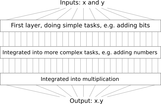
Whenever you are asked to do any complex task, you usually break it down to subtasks and solve the component subtasks. For instance, suppose you’re designing a logical circuit to multiply two numbers. Chances are your circuit will look something like this:
Figure: Logical circuit for multiplication.
Source.
Similarly deep neural networks (i.e lot of layers) can build up multiple layers of abstraction. Consider the following network:
Figure: Deep Neural Network.
Source.
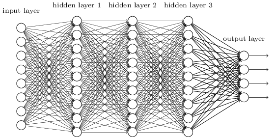
If we’re doing visual pattern recognition, then the neurons in the first layer might learn to recognize edges, the neurons in the second layer could learn to recognize more complex shapes, say triangle or rectangles, built up from edges. The third layer would then recognize still more complex shapes. And so on. These multiple layers of abstraction seem likely to give deep networks a compelling advantage in learning to solve complex pattern recognition problems.
How do we train such deep networks? Stochastic gradient descent as usual. But we’ll run into trouble, with our deep networks not performing much (if at all) better than shallow networks.
Let’s try to understand why are deep networks hard to train:
- Consider the number of parameters in the network. They are huge! If we have to connect 1000 unit hidden layer to 224x224 (50,176) image, we have $65,536*1000 \approx 50e6$ parameters in that layer alone! There are so many parameters that network can easily overfit on the data without generalization.
- Gradients are unstable. Recall the expression for the gradients, $\frac{\partial C}{\partial \theta_l} = \frac{\partial y_L}{\partial u_L} * \frac{\partial y_{L-1}}{\partial u_{L-1}} * \cdots * \frac{\partial y_{l-1}}{\partial u_{l-1}} * \frac{\partial y_l}{\partial \theta_l}$. If few of $\frac{\partial y_m}{\partial u_m} \ll 1$, they will multiply up and make $\frac{\partial C}{\partial \theta_l} \approx 0$. Similarly if few of $\frac{\partial y_m}{\partial u_m} \gg 1$, they make $\frac{\partial C}{\partial \theta_l} \to \infty$. This is the reason why sigmoids are avoided. For sigmoid, $\frac{\partial y}{\partial u} = \frac{d \sigma}{d z}|_{z=u}$ is close to zero if $u$ is either too large or too small. It’s maximum is only $1/4$
Keep these two points in mind. We will see several approaches to deep learning that to some extent manage to overcome or route around these.
Continue reading Part 2.